Evaluating model fit

For Bayesian diagnostic classification models

W. Jake Thompson, Ph.D.

Who am I?

W. Jake Thompson, Ph.D.

• Assistant Director of Psychometrics
  • ATLAS | University of Kansas
• Research: Applications of diagnostic psychometric models
  • Lead psychometrician and Co-PI for the Dynamic Learnings Maps assessments
  • PI for an IES-funded project to develop software for diagnostic models

  @wjakethompson
  wjakethompson.com

Acknowledgements

The research reported here was supported by the Institute of Education Sciences, U.S. Department of Education, through Grant R305D210045 to the University of Kansas. The opinions expressed are those of the authors and do not represent the views of the the Institute or the U.S. Department of Education.

Model fit for DCMs

• Absolute fit: How well does a model fit the data?

  • Model-level (global) fit
  • Item-level fit
    
  • Person-level fit

• Relative fit: How well does a model fit compared to another model?

• Different methods available depending on how the model was estimated (e.g., maximum likelihood, MCMC)

Absolute fit with limited-information indices

• Categorical response data create sparse data matrices

  • 20 binary items: 2²⁰ = 1,048,576 response patterns

• Limited-information indices use lower-order summaries of the contingencies tables (Maydue-Olivares & Joe, 2005)

• Most popular method for model fit in DCMs is the M₂ (Hansen et al., 2016; Liu et al., 2016)

  • p-value < .05 indicates poor model fit

Bayesian absolute fit

• Not constrained to limited-information indices

• Posterior predictive model checks (PPMCs)

  • Generate new data sets from the posterior distribution
  • Calculate summary statistics for each generated data set
  • Compare the distribution to the observed value of the summary statistic

• In this study, we examine a PPMC of the the raw score distribution (Park et al., 2015; Thompson, 2019)

  • 0.025 < ppp < 0.975 indicates good model fit

Relative fit

• Information criteria such as the AIC (Akaike, 1973), BIC (Schwarz, 1978), or similar

• Compare the information criteria for each competing model

  • Index with the lowest value is preferred

• These methods are often inappropriate when using a Bayesian estimation process (e.g., MCMC; Hollenbach & Montgomery, 2020)

Bayesian relative fit

• Information criteria that are designed for Bayesian estimation methods

• Leave-one-out (LOO) cross validation with Pareto-smoothed importance sampling (Vehtari et al., 2017)

  • Asymptotically equivalent to the widely applicable information criterion (WAIC; Watanabe, 2010), but performs better in a wider range of conditions (Gelman et al., 2014).

• As with more traditional methods, we compare the LOO for each competing model

  • Index with the lowest value is preferred
  • Can also calculate the standard error of the difference to help determine if the difference is meaningful

State of the field

• Assessment of model fit is primarily limited to methods that rely on point estimates (e.g., M₂, AIC, BIC)

• Research has not compared the efficacy of Bayesian measures of model fit to the more commonly used measures

• Recent software advances have made Bayesian estimation of DCMs more accessible to applied researchers

  • blatent (Templin, 2023)
  • measr (Thompson, 2024)

The current study

• Simulation study to evaluate the efficacy of Bayesian measures of model fit

• Research questions:

  1. Do Bayesian measures provide an accurate assessment of model fit?
  2. How does the accuracy compare to more common methods for assessing model fit (e.g., M₂)?

Preprint

Simulation design

• 8 test design conditions
  • Attributes: 2 or 3
  • Items per attribute: 5 or 7
  • Sample size: 500 or 1,000
• Within each test design condition, we manipulated the data-generating and estimated model, for 4 total modeling conditions
  • Loglinear cognitive diagnostic model (LCDM; Henson et al., 2009)
  • Deterministic-input, noisy “and” gate (DINA; de la Torre & Douglas, 2004)
• 32 conditions total, each repeated 50 times

Expected outcomes

Generating model	Estimated model	Absolute-fit flag	Relative-fit preference
DINA	DINA	No	DINA
DINA	LCDM	No	DINA
LCDM	DINA	Yes	LCDM
LCDM	LCDM	No	LCDM

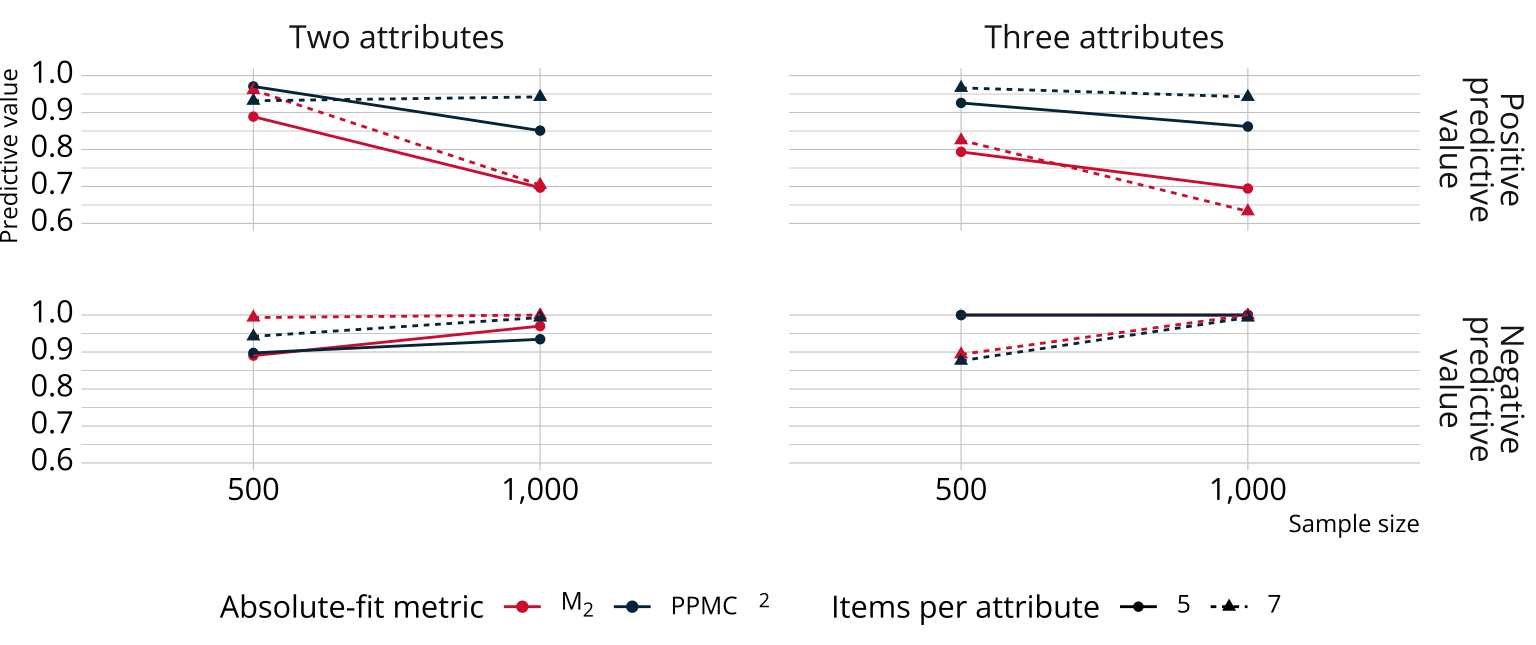
Results: Absolute fit

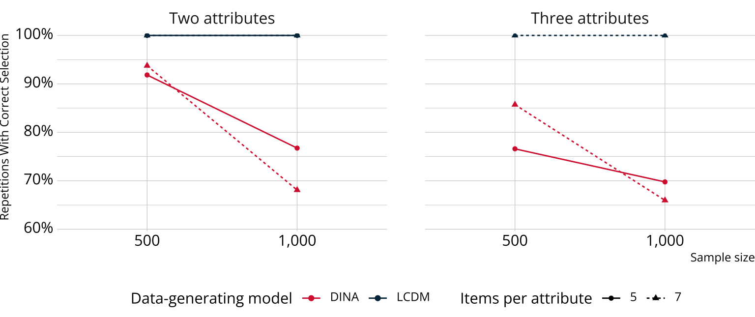
Results: Relative fit

Conclusions

• Bayesian methods performed as well or better for absolute fit

• Bayesian methods for relative fit performed as well or better than has been reported for other non-Bayesian information criteria

• Future directions

  • Larger, more complex test designs
  • Comparison to additional metrics (e.g., RMSEA, SRMSR)

Learn more about measr

measr documentation

wjakethompson/measr

Thank you!

Slides

 wjakethompson.com
 wjakethompson@ku.edu
 in/wjakethompson
 @wjakethompson
 @wjakethompson@fosstodon.org
 @wjakethompson.com
 @wjakethompson
 @wjakethompson

Appendix: Calculating the PPMC
raw score distribution χ²

PPMC: Raw score by iteration

• For each iteration, calculate the total number of respondents at each score point

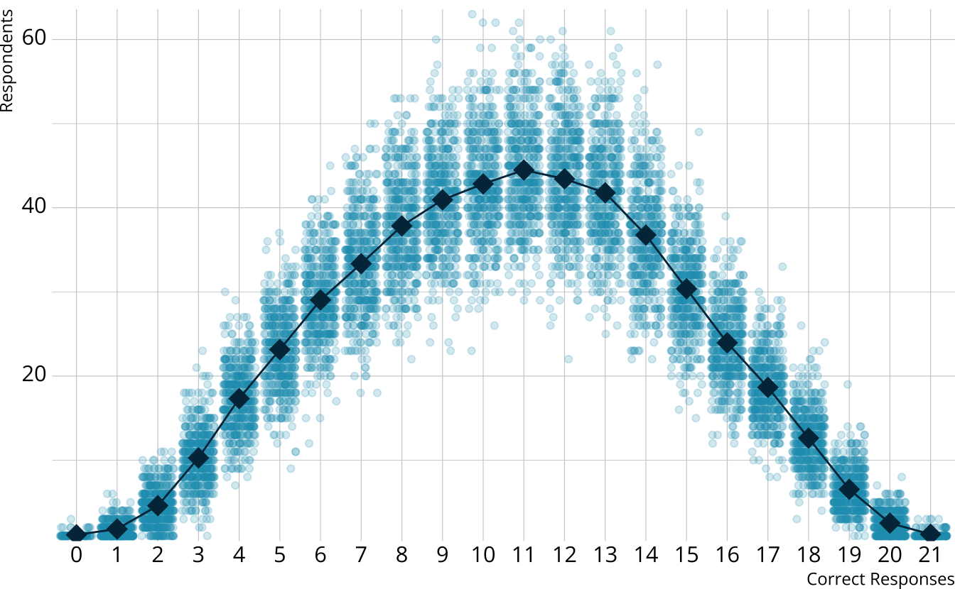
PPMC: Expected counts, by raw score

• For each iteration, calculate the total number of respondents at each score point

• Calculate the expected number of respondents at each score point

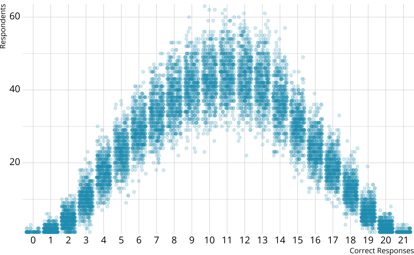
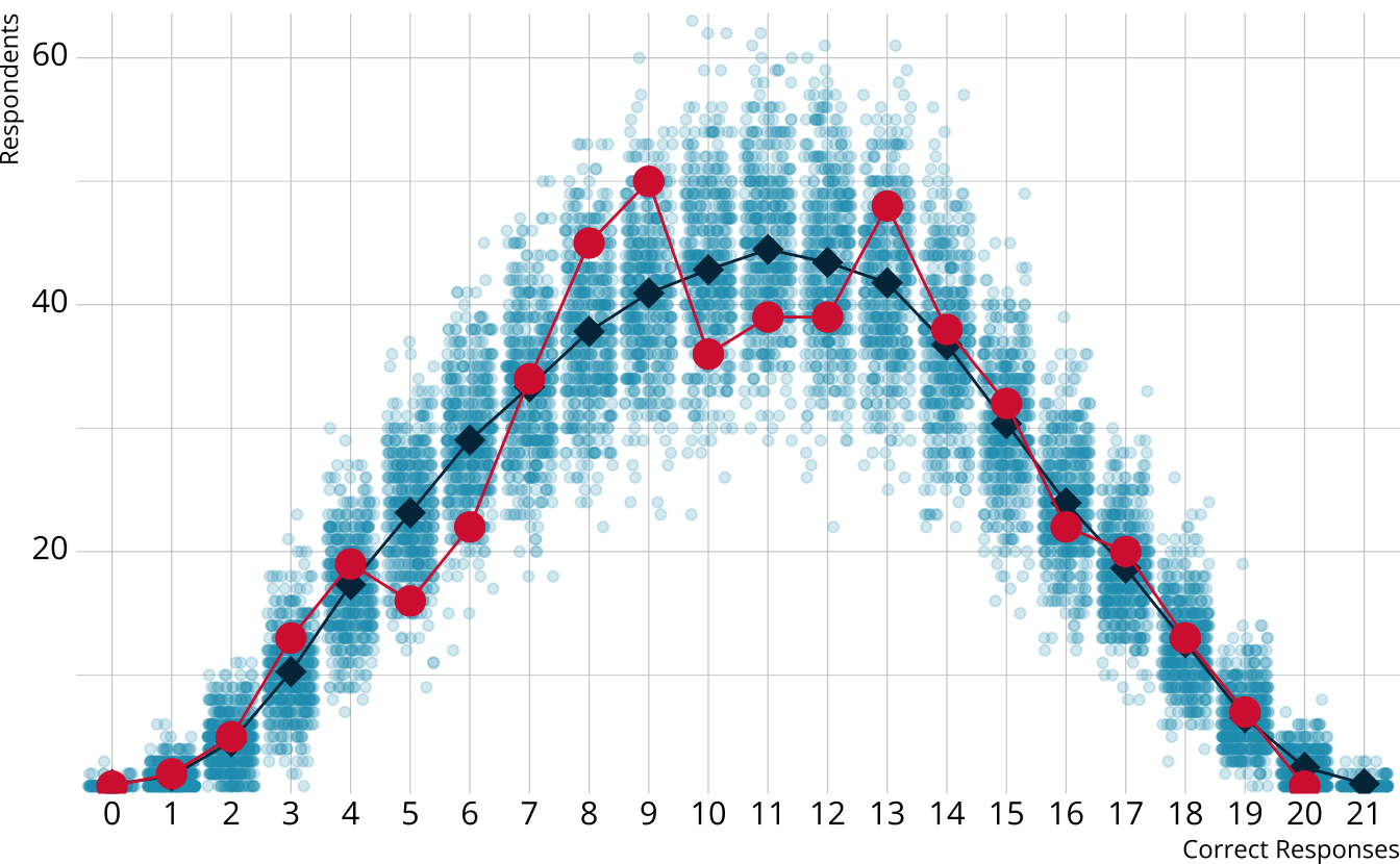
PPMC: Observed counts

• For each iteration, calculate the total number of respondents at each score point

• Calculate the expected number of respondents at each score point

• Calculate the observed number of respondents at each score point

PPMC: χ² summary statistic

• For each replication, calculate a χ²_rep statistic

#> # A tibble: 22 × 4
#>    .draw score replication_n expected
#>    <int> <int>         <int>    <dbl>
#>  1    13     1             2     1.82
#>  2    13     2             6     4.59
#>  3    13     3            18    10.3 
#>  4    13     4             9    17.3 
#>  5    13     5            19    23.1 
#>  6    13     6            29    29.0 
#>  7    13     7            34    33.4 
#>  8    13     8            39    37.8 
#>  9    13     9            39    40.9 
#> 10    13    10            38    42.8 
#> # ℹ 12 more rows

\[ \chi^2_{rep} = \sum_{s=0}^S\frac{[n_s - E(n_s)]^2}{E(n_s)} \]

#> [1] 25.26204

PPMC: χ² distribution

• For each replication, calculate a χ²_rep statistic

• Create a distribution of the expected value of the χ² statistic

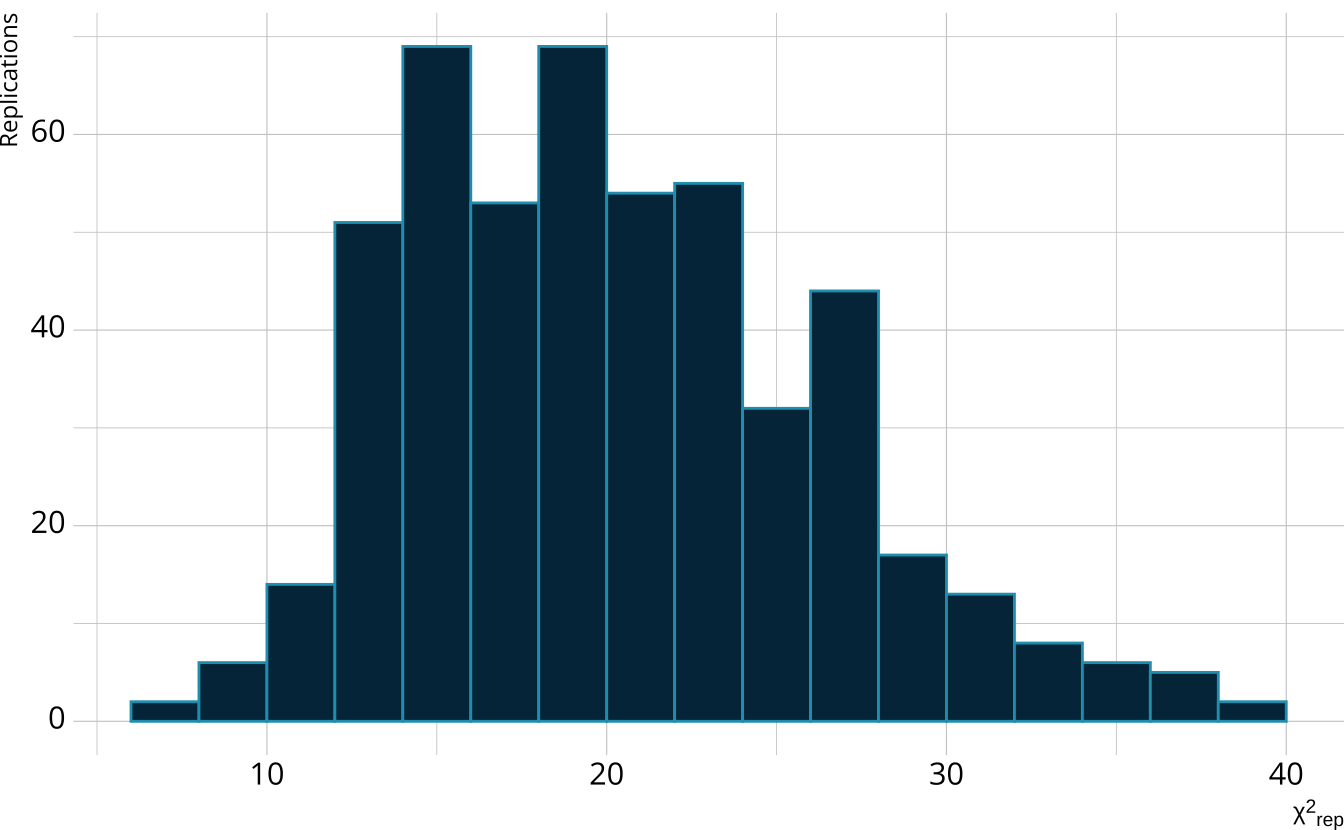
PPMC: χ² observed value

• For each replication, calculate a χ²_rep statistic

• Create a distribution of the expected value of the χ² statistic

• Calculate the χ² value comparing the observed data to the expectation

PPMC: Posterior predictive p-value

• Calculate the proportion of χ²_rep draws greater than our observed value

• Flag if the observed value is outside a predefined boundary (e.g., .025 < ppp < 0.975)

• In our example ppp = 0.856